In this post we are going to develop a neural network forex trading system. We will use a simple neural network called NNET. In recent years, artificial intelligence and deep learning has taken over the trading world. Hedge funds and big banks are using these advanced cutting edge tools to beat the market on a daily basis. On the other hand, most retail traders have no clue what this deep learning thing is and how they can use artificial intelligence in trading. Have you noticed one thing in the past few years? Traditional technical analysis tools like MACD, Stochastic, CCI, Bollinger Bands don’t work like they used to work in the past. But one thing still works. That is price action that includes candlestick patterns. Did you read the post on a USDJPY trade that made 600 pips with a 10 pip stop loss? I use price action a lot in my trading. The key is to keep the risk as low as possible.
Time has come for you to start learning and using these new tools that big Wall Street firms are already using. In the last few years there has been a tremendous explosion in the computational power of computers. This has made it possible to use sophisticated data mining algorithmis to make predictions on market behavior. Neural Networks were developed many decades back. Neural networks work just like the human brain neurons. When there is a signal. it can only fire the neuron if it has sufficient strength. This is how the human brain does all its work. Neural networks also work on the same principle. If we have an input signal, it should be above a certain threshold to trigger an output signal. Now there are many neural network software that are being sold in the market. You can buy a good neural network software from $500 to $2,000. It is easy to use these software as everything has been done for you. But I will take a different approach here. Instead of buying an expensive neural network software I suggest you develop your own neural network trading systems. So we will be developing a neural network forex trading system in this post. Keep on reading if you want to learn how to do it. Did you read this post on how to predict gold price using kernel ridge regression?
It might take you a few months to learn the theory behind neural networks but it will be worth the effort. Once you have developed the art of training neural network models, you can use it in any field. So if you are interested in knowing how these models are developed keep on reading this post. You should learn R as well as Python. R and Python are powerful data science scripting languages that allow you to do a lot of financial modelling that you cannot do in Excel. Time series analysis is very important when it comes to financial modelling. Price is a financial time series. We record the closing price after every 1 hour or 4 hours regularly. This sequence of closing price constitutes a time series. We as traders know that past price can be used to predict the future price. This is precisely what time series analysis also assumes. We can use past price to predict future price using autoregressive models. I have developed a course on Time Series Analysis for Traders that you can take a look at. Many traders have no idea how to use time series models in their trading. I show you how to use time series models in your trading and get great results.
Both R and Python are easy to learn. With a little effort you can learn these languages. In this post we will be using R. R is a powerful statistical language that is used widely in academia. You should R installed on your computer as well as RStudio. Both are open source. So you don’t have to pay anything for using R. I have developed a course on Python Machine Learning for Traders. In this course I show you how to develop different machine learning models for your trading system using Python. As said in the start algorithmic trading has become very popular now a days. Days of manual trading are coming to an end. You should start learning fundamentals of algorithmic trading. Today more than 80% of the trades that are being placed at Wall Street are being placed by algorithms. 21st century is being called the century of algorithms. Algorithms are revolutionizing all field of life from health, medicine, car driving, aeroplane flying, detecting bank frauds and all sorts of things. I have developed this course on Algorithmic Trading with Python that you can take a look at. Don’t worry I have also developed courses on R that traders can use.
Now when you develop a neural network model, feature selection is very important. Features are the inputs that you give to the model to do the calculations and make predictions. I have been trading for many years now and know the importance of candlesticks as said above. Candlestick patterns are good leading signals. Candlestick patterns are mostly 2 stick patterns and 3 stick patterns. So we will use Open, High, Low and Close of the price to develop features that try to model candlesticks. We will see if we can use these features to predict the market. We will be using high frequency data especially M1 timeframe. Yes, I am talking about 1 minute timeframe. Did you check this trend following high frequency trading system? The model that we develop can be used on other timeframes also like the 15 minute, 30 minute, 60 minute, 240 minute. We can do that later. If we can predict the price after each 5 minutes with lets say 80% accuracy we can use that knowledge to trade 5 minute forex binary options as well. Below is the candlestick chart of the 1 minute GBPUSD data.
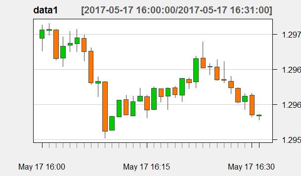
As you can see R can make very beautiful candlestick charts very fast. If you have a quadcore computer than you can make R even more fast by using Microsoft R Open. I explain eerything how to do it in my course on R. The idea behind using high frequency data was that I wanted to show how fast we can do the calculations and make the predictions using R. I will develop three Neural Network Forex Trading Models .
Neural Network Forex Trading System 1
In the first model we take the closing price as feature number 1. We then use it to develop features like (Close-Open)/Open and (high-Low)/Low. Now we lag these 3 input features 1 time and 2 time so that we have a total of 9 input features. We will use a simple neural network model known as a feed forward neural network with one hidden layer. The hidden layer has got 10 neurons. Lets’ see if we get a model that can make good predictions. Below is the R code.
> library(quantmod)
Loading required package: xts
Loading required package: zoo

Attaching package: ‘zoo’

The following objects are masked from ‘package:base’:

    as.Date, as.Date.numeric

Loading required package: TTR
Version 0.4-0 included new data defaults. See ?getSymbols.
> data <- read.csv("D:/MarketData/GBPUSD+1.csv", header = FALSE)
> colnames(data) <- c("Date", "Time", "Open", "High", "Low", "Close", "Volume")
> data1 <- as.xts(data[,-(1:2)], as.POSIXct(paste(data[,1],data[,2]),
+                                           format='%Y.%m.%d %H:%M'))
> tail(data1)
                       Open    High     Low   Close Volume
2017-05-17 16:26:00 1.29636 1.29661 1.29631 1.29634    215
2017-05-17 16:27:00 1.29633 1.29640 1.29615 1.29624    144
2017-05-17 16:28:00 1.29623 1.29624 1.29602 1.29603    195
2017-05-17 16:29:00 1.29604 1.29615 1.29593 1.29612    234
2017-05-17 16:30:00 1.29613 1.29616 1.29582 1.29585    234
2017-05-17 16:31:00 1.29584 1.29586 1.29578 1.29585     46
> data2<- data1[,"Close"]
> data2$CO <- (data1[, "Close"]-data1[,"Open"])/data1[,"Open"]
> data2$HL <- (data1[, "High"]-data1[,"Low"])/data1[,"Low"]
> data2$Close1 <- lag(data2$Close, k=1)
> data2$CO1 <- lag(data2$CO, k=1)
> data2$HL1 <- lag(data2$HL, k=1)
> data2$Close2 <- lag(data2$Close, k=2)
> data2$CO2 <- lag(data2$CO, k=2)
> data2$HL2 <- lag(data2$HL, k=2)
> tail(data2)
                      Close            CO           HL  Close1           CO1          HL1
2017-05-17 16:26:00 1.29634 -1.542781e-05 2.314261e-04 1.29635 -1.388321e-04 0.0002314208
2017-05-17 16:27:00 1.29624 -6.942677e-05 1.928789e-04 1.29634 -1.542781e-05 0.0002314261
2017-05-17 16:28:00 1.29603 -1.542936e-04 1.697505e-04 1.29624 -6.942677e-05 0.0001928789
2017-05-17 16:29:00 1.29612  6.172649e-05 1.697623e-04 1.29603 -1.542936e-04 0.0001697505
2017-05-17 16:30:00 1.29585 -2.160277e-04 2.623821e-04 1.29612  6.172649e-05 0.0001697623
2017-05-17 16:31:00 1.29585  7.717002e-06 6.173888e-05 1.29585 -2.160277e-04 0.0002623821
                     Close2           CO2          HL2
2017-05-17 16:26:00 1.29654  7.712895e-06 0.0001234168
2017-05-17 16:27:00 1.29635 -1.388321e-04 0.0002314208
2017-05-17 16:28:00 1.29634 -1.542781e-05 0.0002314261
2017-05-17 16:29:00 1.29624 -6.942677e-05 0.0001928789
2017-05-17 16:30:00 1.29603 -1.542936e-04 0.0001697505
2017-05-17 16:31:00 1.29612  6.172649e-05 0.0001697623
> pips<- 10000*(diff(data1$Close, k=5))
> n=2
> direction <- ifelse(pips > n, "Up",
+                          ifelse(pips < -n, "Down", "Range"))
> direction <- lag(direction, k=-5)
> tail(direction)
                    Close
2017-05-17 16:26:00 "Range"
2017-05-17 16:27:00 NA
2017-05-17 16:28:00 NA
2017-05-17 16:29:00 NA
2017-05-17 16:30:00 NA
2017-05-17 16:31:00 NA
> direction <- factor(direction)
> x <- nrow(data2)
> train2<- data2[(x-300):(x-100),]
> valid2<- data2[(x-99):(x-6),]
> test2<- data2[(x-5):x,]
> trainmean<- apply(train2,2,mean)
> trainstd<- apply(train2,2,sd)
> trainidn<- (matrix(1,dim(train2)[1],dim(train2)[2]))
> valiidn<- (matrix(1,dim(valid2)[1],dim(valid2)[2]))
> testidn<- (matrix(1,dim(test2)[1],dim(test2)[2]))
> norm_train<- (train2 - t(trainmean*t(trainidn))) / t(trainstd*t(trainidn))
> norm_valid<- (valid2 - t(trainmean*t(valiidn))) / t(trainstd*t(valiidn))
> norm_test<- (test2 - t(trainmean*t(testidn))) / t(trainstd*t(testidn))
> traindir<- direction[(x-300):(x-100)]
> validir<- direction[(x-99):(x-6)]
> testdir<- direction[(x-5):x]
> library(caret)
Loading required package: lattice
Loading required package: ggplot2
> library(e1071)
> m3 <- train(norm_train, traindir,
+             method = "nnet",
+             tuneGrid = expand.grid(
+               .size = c(10),
+               .decay = 0.1),
+             trControl = trainControl(method = "none"),
+             MaxNWts = 50000,
+             maxit = 1000)
Loading required package: nnet
# weights:  133
initial  value 342.317162
iter  10 value 114.701962
iter  20 value 101.922012
iter  30 value 95.614864
iter  40 value 92.497605
iter  50 value 90.573152
iter  60 value 89.866768
iter  70 value 89.506106
iter  80 value 89.417506
iter  90 value 89.384365
iter 100 value 89.375842
iter 110 value 89.374413
iter 120 value 89.366938
iter 130 value 89.365762
final  value 89.365750
converged
We have developed a neural network model which is very simple. it consists of only one hidden layer with 10 neurons. Firsst we check how well the model trained on the training data. We divided the data into training data and validation data. Training data was used to train the neural network.Let’s check how well it has trained itself on the training data.
> direction1 <- predict(m3)
> caret::confusionMatrix(xtabs(~direction1 + traindir))
Confusion Matrix and Statistics

          traindir
direction1 Down Range  Up
     Down     7     0   0
     Range    8   163  13
     Up       0     0  10

Overall Statistics

               Accuracy : 0.8955
                 95% CI : (0.8447, 0.9342)
    No Information Rate : 0.8109
    P-Value [Acc > NIR] : 0.0007871

                  Kappa : 0.581
 Mcnemar's Test P-Value : NA

Statistics by Class:

                     Class: Down Class: Range Class: Up
Sensitivity              0.46667       1.0000   0.43478
Specificity              1.00000       0.4474   1.00000
Pos Pred Value           1.00000       0.8859   1.00000
Neg Pred Value           0.95876       1.0000   0.93194
Prevalence               0.07463       0.8109   0.11443
Detection Rate           0.03483       0.8109   0.04975
Detection Prevalence     0.03483       0.9154   0.04975
Balanced Accuracy        0.73333       0.7237   0.71739
Now you can see above our neural network model has trained well. It is giving an accuracy off 89% on the training data. We will call it in sample accuracy. What we want is our model to predict on unseen data and check what is the accuracy level. This is known as out of sample accuracy. So we use data that we call validation data that our model has not seen and see the accuracy that it is giving. Did you read the post on why it is difficult to predict exchange rates using statistical models?
> vali_pred <- predict(m3, norm_valid)
> head(vali_pred)
[1] Range Range Range Range Range Range
Levels: Down Range Up
> barplot(table(direction))
> caret::confusionMatrix(xtabs(~vali_pred + validir))
Confusion Matrix and Statistics

         validir
vali_pred Down Range Up
    Down     0     1  0
    Range    7    68 11
    Up       1     6  0

Overall Statistics

               Accuracy : 0.7234
                 95% CI : (0.6215, 0.8107)
    No Information Rate : 0.7979
    P-Value [Acc > NIR] : 0.96923

                  Kappa : -0.0621
 Mcnemar's Test P-Value : 0.07284

Statistics by Class:

                     Class: Down Class: Range Class: Up
Sensitivity              0.00000      0.90667   0.00000
Specificity              0.98837      0.05263   0.91566
Pos Pred Value           0.00000      0.79070   0.00000
Neg Pred Value           0.91398      0.12500   0.87356
Prevalence               0.08511      0.79787   0.11702
Detection Rate           0.00000      0.72340   0.00000
Detection Prevalence     0.01064      0.91489   0.07447
Balanced Accuracy        0.49419      0.47965   0.45783
You can see the accuracy of our model has dropped from 89% to 72% when we switch from seen data to unseen data. Can we do something to increase our accuracy level on unseen data? In the above model we have lagged our input features 3 times, lets do it 5 times and see if it helps in improving accuracy.
Neural Network Forex Trading System 2
As said above we increased the inputs by lagging the input features 2 more time. Model building is all trial and error. We need a lot of patience to build a good model. We have expert knowledge regarding our field which is the currency market in this case. We know candlestick patterns have predictive power. We also know looking at the past 4-5 candles we can predict in which direction market is going to move. So lets; use 5 lags in this improved model and see if we can increase the accuracy for our out of sample model. Out of sample data is very important for us as it is unseen and its acccuracy will tell us how much success rate we can expect from our trading system based on that model. We have divided market movement into 3 classes. Movement below 2 pips will be classed as ranging. Movement above 2 pips will be classed as Up and movement below 2 pips will be classed as down movement.
> #load the libraries
> library(quantmod)
> #import the data
> data <- read.csv("D:/MarketData/GBPUSD+1.csv", header = FALSE)
> colnames(data) <- c("Date", "Time", "Open", "High", "Low", "Close", "Volume")
> #convert dataframe to an xts object
> data1 <- as.xts(data[,-(1:2)], as.POSIXct(paste(data[,1],data[,2]),
+                                           format='%Y.%m.%d %H:%M'))
>
> tail(data1)
                       Open    High     Low   Close Volume
2017-05-17 16:26:00 1.29636 1.29661 1.29631 1.29634    215
2017-05-17 16:27:00 1.29633 1.29640 1.29615 1.29624    144
2017-05-17 16:28:00 1.29623 1.29624 1.29602 1.29603    195
2017-05-17 16:29:00 1.29604 1.29615 1.29593 1.29612    234
2017-05-17 16:30:00 1.29613 1.29616 1.29582 1.29585    234
2017-05-17 16:31:00 1.29584 1.29586 1.29578 1.29585     46
>
> data2<- data1[,"Close"]
> data2$CO <- (data1[, "Close"]-data1[,"Open"])/data1[,"Open"]
> data2$HL <- (data1[, "High"]-data1[,"Low"])/data1[,"Low"]
> data2$Close1 <- lag(data2$Close, k=1)
> data2$CO1 <- lag(data2$CO, k=1)
> data2$HL1 <- lag(data2$HL, k=1)
> data2$Close2 <- lag(data2$Close, k=2)
> data2$CO2 <- lag(data2$CO, k=2)
> data2$HL2 <- lag(data2$HL, k=2)
> data2$Close3 <- lag(data2$Close, k=3)
> data2$CO3 <- lag(data2$CO, k=3)
> data2$HL3 <- lag(data2$HL, k=3)
> data2$Close4 <- lag(data2$Close, k=4)
> data2$CO4 <- lag(data2$CO, k=4)
> data2$HL4 <- lag(data2$HL, k=4)
> tail(data2)
                      Close            CO           HL  Close1           CO1          HL1
2017-05-17 16:26:00 1.29634 -1.542781e-05 2.314261e-04 1.29635 -1.388321e-04 0.0002314208
2017-05-17 16:27:00 1.29624 -6.942677e-05 1.928789e-04 1.29634 -1.542781e-05 0.0002314261
2017-05-17 16:28:00 1.29603 -1.542936e-04 1.697505e-04 1.29624 -6.942677e-05 0.0001928789
2017-05-17 16:29:00 1.29612  6.172649e-05 1.697623e-04 1.29603 -1.542936e-04 0.0001697505
2017-05-17 16:30:00 1.29585 -2.160277e-04 2.623821e-04 1.29612  6.172649e-05 0.0001697623
2017-05-17 16:31:00 1.29585  7.717002e-06 6.173888e-05 1.29585 -2.160277e-04 0.0002623821
                     Close2           CO2          HL2  Close3           CO3          HL3
2017-05-17 16:26:00 1.29654  7.712895e-06 0.0001234168 1.29652 -1.079697e-04 0.0002853793
2017-05-17 16:27:00 1.29635 -1.388321e-04 0.0002314208 1.29654  7.712895e-06 0.0001234168
2017-05-17 16:28:00 1.29634 -1.542781e-05 0.0002314261 1.29635 -1.388321e-04 0.0002314208
2017-05-17 16:29:00 1.29624 -6.942677e-05 0.0001928789 1.29634 -1.542781e-05 0.0002314261
2017-05-17 16:30:00 1.29603 -1.542936e-04 0.0001697505 1.29624 -6.942677e-05 0.0001928789
2017-05-17 16:31:00 1.29612  6.172649e-05 0.0001697623 1.29603 -1.542936e-04 0.0001697505
                     Close4           CO4          HL4
2017-05-17 16:26:00 1.29665  2.545668e-04 0.0003471579
2017-05-17 16:27:00 1.29652 -1.079697e-04 0.0002853793
2017-05-17 16:28:00 1.29654  7.712895e-06 0.0001234168
2017-05-17 16:29:00 1.29635 -1.388321e-04 0.0002314208
2017-05-17 16:30:00 1.29634 -1.542781e-05 0.0002314261
2017-05-17 16:31:00 1.29624 -6.942677e-05 0.0001928789
>
> #direction<- data.frame(matrix(NA,dim(data2)[1],1))
> pips<- 10000*(diff(data1$Close, k=5))
> n=2
> direction <- ifelse(pips > n, "Up",
+                     ifelse(pips < -n, "Down", "Range"))
>
> direction <- lag(direction, k=-5)
> tail(direction)
                    Close
2017-05-17 16:26:00 "Range"
2017-05-17 16:27:00 NA
2017-05-17 16:28:00 NA
2017-05-17 16:29:00 NA
2017-05-17 16:30:00 NA
2017-05-17 16:31:00 NA
> direction <- factor(direction)
>
> x <- nrow(data2)
>
> train2<- data2[(x-500):(x-200),]
> valid2<- data2[(x-199):(x-6),]
> test2<- data2[(x-5):x,]
>
>
> trainmean<- apply(train2,2,mean)
> trainstd<- apply(train2,2,sd)
>
>
> trainidn<- (matrix(1,dim(train2)[1],dim(train2)[2]))
> valiidn<- (matrix(1,dim(valid2)[1],dim(valid2)[2]))
> testidn<- (matrix(1,dim(test2)[1],dim(test2)[2]))
>
>
> norm_train<- (train2 - t(trainmean*t(trainidn))) / t(trainstd*t(trainidn))
> norm_valid<- (valid2 - t(trainmean*t(valiidn))) / t(trainstd*t(valiidn))
> norm_test<- (test2 - t(trainmean*t(testidn))) / t(trainstd*t(testidn))
>
>
> traindir<- direction[(x-500):(x-200)]
> validir<- direction[(x-199):(x-6)]
> testdir<- direction[(x-5):x]
>
> library(caret)
> library(e1071)
> m3 <- train(norm_train, traindir,
+             method = "nnet",
+             tuneGrid = expand.grid(
+               .size = c(40),
+               .decay = 0.1),
+             trControl = trainControl(method = "none"),
+             MaxNWts = 50000,
+             maxit = 1000)
# weights:  763
initial  value 508.087290
iter  10 value 214.118369
iter  20 value 163.135688
iter  30 value 133.087117
iter  40 value 116.461972
iter  50 value 110.088698
iter  60 value 105.385186
iter  70 value 103.180276
iter  80 value 102.339347
iter  90 value 101.762369
iter 100 value 100.844553
iter 110 value 100.235618
iter 120 value 99.877796
iter 130 value 99.623222
iter 140 value 99.450404
iter 150 value 99.301965
iter 160 value 99.256903
iter 170 value 99.185848
iter 180 value 99.115716
iter 190 value 99.007136
iter 200 value 98.988401
iter 210 value 98.974478
iter 220 value 98.966304
iter 230 value 98.962196
iter 240 value 98.958897
iter 250 value 98.956157
iter 260 value 98.954591
iter 270 value 98.953682
iter 280 value 98.953133
iter 290 value 98.951986
iter 300 value 98.941686
iter 310 value 98.916859
iter 320 value 98.887349
iter 330 value 98.876204
iter 340 value 98.871270
iter 350 value 98.867634
iter 360 value 98.861265
iter 370 value 98.859520
iter 380 value 98.857350
iter 390 value 98.809161
iter 400 value 98.794699
iter 410 value 98.791562
iter 420 value 98.790035
iter 430 value 98.789596
iter 440 value 98.789251
iter 450 value 98.788956
iter 460 value 98.788709
iter 470 value 98.788521
iter 480 value 98.788423
iter 490 value 98.788364
iter 500 value 98.788318
iter 510 value 98.788301
final  value 98.788299
converged
>
> #calculate acccuracy on the training data
> direction1 <- predict(m3)
> caret::confusionMatrix(xtabs(~direction1 + traindir))
Confusion Matrix and Statistics

          traindir
direction1 Down Range  Up
     Down    33     0   0
     Range    0   228   1
     Up       0     0  39

Overall Statistics

               Accuracy : 0.9967
                 95% CI : (0.9816, 0.9999)
    No Information Rate : 0.7575
    P-Value [Acc > NIR] : < 2.2e-16

                  Kappa : 0.9916
 Mcnemar's Test P-Value : NA

Statistics by Class:

                     Class: Down Class: Range Class: Up
Sensitivity               1.0000       1.0000    0.9750
Specificity               1.0000       0.9863    1.0000
Pos Pred Value            1.0000       0.9956    1.0000
Neg Pred Value            1.0000       1.0000    0.9962
Prevalence                0.1096       0.7575    0.1329
Detection Rate            0.1096       0.7575    0.1296
Detection Prevalence      0.1096       0.7608    0.1296
Balanced Accuracy         1.0000       0.9932    0.9875
>
> #calculate accuracy on validation data
> vali_pred <- predict(m3, norm_valid)
> head(vali_pred)
[1] Range Range Range Range Range Range
Levels: Down Range Up
> barplot(table(direction))
> caret::confusionMatrix(xtabs(~vali_pred + validir))
Confusion Matrix and Statistics

         validir
vali_pred Down Range  Up
    Down     1     9   0
    Range   11   152  17
    Up       2     1   1

Overall Statistics

               Accuracy : 0.7938
                 95% CI : (0.73, 0.8484)
    No Information Rate : 0.8351
    P-Value [Acc > NIR] : 0.9465680

                  Kappa : 0.061
 Mcnemar's Test P-Value : 0.0009289

Statistics by Class:

                     Class: Down Class: Range Class: Up
Sensitivity             0.071429       0.9383  0.055556
Specificity             0.950000       0.1250  0.982955
Pos Pred Value          0.100000       0.8444  0.250000
Neg Pred Value          0.929348       0.2857  0.910526
Prevalence              0.072165       0.8351  0.092784
Detection Rate          0.005155       0.7835  0.005155
Detection Prevalence    0.051546       0.9278  0.020619
Balanced Accuracy       0.510714       0.5316  0.519255
In the above model we increased the hidden layer neurons from 10 to 40 plus we increased the inputs from 12 to 16. This increased the in sample accuracy from 89% to 99% while out of sample accuracy increased from 72% to 79%. We want an out of sample accuracy of 85% at least before we start trading live with our model. We try to re-engineer the features and see if it helps.
Neural Network Forex Trading System 3
This is our third model. In this model we will be using candlestick pattern concepts like the candlestick body which is just close minue open and the candlestick range which is just the high minus low. We will also use concept of Upper Shadow which is the difference between the High and the Close for a bullish candle and High and the Low for a bearish candle for a calculating the Upper Shadow. For the Lower Shadow we take the difference between the Open and Low for a bullish candle and Close and Low for a bearish candle.
> #load the libraries
> library(quantmod)
> #import the data
> data <- read.csv("D:/MarketData/GBPUSD+1.csv", header = FALSE)
> colnames(data) <- c("Date", "Time", "Open", "High", "Low", "Close", "Volume")
> #convert dataframe to an xts object
> data1 <- as.xts(data[,-(1:2)], as.POSIXct(paste(data[,1],data[,2]),
+                                           format='%Y.%m.%d %H:%M'))
>
> tail(data1)
                       Open    High     Low   Close Volume
2017-05-17 16:26:00 1.29636 1.29661 1.29631 1.29634    215
2017-05-17 16:27:00 1.29633 1.29640 1.29615 1.29624    144
2017-05-17 16:28:00 1.29623 1.29624 1.29602 1.29603    195
2017-05-17 16:29:00 1.29604 1.29615 1.29593 1.29612    234
2017-05-17 16:30:00 1.29613 1.29616 1.29582 1.29585    234
2017-05-17 16:31:00 1.29584 1.29586 1.29578 1.29585     46
>
> data2<- data1[,"Close"]
> data2$Body <- data1[, "Close"]-data1[,"Open"]
> data2$Range <- data1[, "High"]-data1[,"Low"]
> data2$US <- ifelse(data1[, "Close"] > data1[ ,"Open"],
+                    data1[, "High"]-data1[, "Close"],
+                    data1[, "High"]-data1[, "Open"])
> data2$LS <- ifelse(data1[, "Close"] > data1[ ,"Open"],
+                    data1[, "Open"]-data1[, "Low"],
+                    data1[, "Close"]-data1[, "Low"])
> data2$Close1 <- lag(data2$Close, k=1)
> data2$Body1 <- lag(data2$Body, k=1)
> data2$Range1 <- lag(data2$Range, k=1)
> data2$US1 <- lag(data2$US, k=1)
> data2$LS1 <- lag(data2$LS, k=1)
> data2$Close2 <- lag(data2$Close, k=2)
> data2$Body2 <- lag(data2$Body, k=2)
> data2$Range2 <- lag(data2$Range, k=2)
> data2$US2 <- lag(data2$US, k=2)
> data2$LS2 <- lag(data2$LS, k=2)
> tail(data2)
                      Close     Body   Range      US      LS  Close1    Body1  Range1     US1
2017-05-17 16:26:00 1.29634 -0.00002 0.00030 0.00025 0.00003 1.29635 -0.00018 0.00030 0.00011
2017-05-17 16:27:00 1.29624 -0.00009 0.00025 0.00007 0.00009 1.29634 -0.00002 0.00030 0.00025
2017-05-17 16:28:00 1.29603 -0.00020 0.00022 0.00001 0.00001 1.29624 -0.00009 0.00025 0.00007
2017-05-17 16:29:00 1.29612  0.00008 0.00022 0.00003 0.00011 1.29603 -0.00020 0.00022 0.00001
2017-05-17 16:30:00 1.29585 -0.00028 0.00034 0.00003 0.00003 1.29612  0.00008 0.00022 0.00003
2017-05-17 16:31:00 1.29585  0.00001 0.00008 0.00001 0.00006 1.29585 -0.00028 0.00034 0.00003
                        LS1  Close2    Body2  Range2     US2     LS2
2017-05-17 16:26:00 0.00001 1.29654  0.00001 0.00016 0.00004 0.00011
2017-05-17 16:27:00 0.00003 1.29635 -0.00018 0.00030 0.00011 0.00001
2017-05-17 16:28:00 0.00009 1.29634 -0.00002 0.00030 0.00025 0.00003
2017-05-17 16:29:00 0.00001 1.29624 -0.00009 0.00025 0.00007 0.00009
2017-05-17 16:30:00 0.00011 1.29603 -0.00020 0.00022 0.00001 0.00001
2017-05-17 16:31:00 0.00003 1.29612  0.00008 0.00022 0.00003 0.00011
>
> #direction<- data.frame(matrix(NA,dim(data2)[1],1))
> pips<- 10000*(diff(data1$Close, k=5))
> n=2.5
> direction <- ifelse(pips > n, "Up",
+                     ifelse(pips < -n, "Down", "Range"))
>
> direction <- lag(direction, k=-5)
> tail(direction)
                    Close
2017-05-17 16:26:00 "Range"
2017-05-17 16:27:00 NA
2017-05-17 16:28:00 NA
2017-05-17 16:29:00 NA
2017-05-17 16:30:00 NA
2017-05-17 16:31:00 NA
> direction <- factor(direction)
>
> x <- nrow(data2)
>
> train2<- data2[(x-300):(x-100),]
> valid2<- data2[(x-99):(x-6),]
> test2<- data2[(x-5):x,]
>
>
> trainmean<- apply(train2,2,mean)
> trainstd<- apply(train2,2,sd)
>
>
> trainidn<- (matrix(1,dim(train2)[1],dim(train2)[2]))
> valiidn<- (matrix(1,dim(valid2)[1],dim(valid2)[2]))
> testidn<- (matrix(1,dim(test2)[1],dim(test2)[2]))
>
>
> norm_train<- (train2 - t(trainmean*t(trainidn))) / t(trainstd*t(trainidn))
> norm_valid<- (valid2 - t(trainmean*t(valiidn))) / t(trainstd*t(valiidn))
> norm_test<- (test2 - t(trainmean*t(testidn))) / t(trainstd*t(testidn))
>
>
> traindir<- direction[(x-300):(x-100)]
> validir<- direction[(x-99):(x-6)]
> testdir<- direction[(x-5):x]
>
> library(caret)
> library(e1071)
> m3 <- train(norm_train, traindir,
+             method = "nnet",
+             tuneGrid = expand.grid(
+               .size = c(10),
+               .decay = 0.1),
+             trControl = trainControl(method = "none"),
+             MaxNWts = 50000,
+             maxit = 1000)
# weights:  193
initial  value 147.861754
iter  10 value 73.658023
iter  20 value 55.491725
iter  30 value 48.026823
iter  40 value 46.252393
iter  50 value 45.742213
iter  60 value 45.279406
iter  70 value 45.071429
iter  80 value 45.004627
iter  90 value 44.975451
iter 100 value 44.908225
iter 110 value 44.851912
iter 120 value 44.682247
iter 130 value 44.633824
iter 140 value 44.577723
iter 150 value 44.481995
iter 160 value 44.344888
iter 170 value 44.071917
iter 180 value 43.951889
iter 190 value 43.923721
iter 200 value 43.919855
iter 210 value 43.919536
final  value 43.919523
converged
>
> # calculate in sample accuracy
> #calculate acccuracy on the training data
> direction1 <- predict(m3)
> caret::confusionMatrix(xtabs(~direction1 + traindir))
Confusion Matrix and Statistics

          traindir
direction1 Down Range  Up
     Down     9     0   0
     Range    1   175   0
     Up       0     0  16

Overall Statistics

               Accuracy : 0.995
                 95% CI : (0.9726, 0.9999)
    No Information Rate : 0.8706
    P-Value [Acc > NIR] : 2.498e-11

                  Kappa : 0.9783
 Mcnemar's Test P-Value : NA

Statistics by Class:

                     Class: Down Class: Range Class: Up
Sensitivity              0.90000       1.0000    1.0000
Specificity              1.00000       0.9615    1.0000
Pos Pred Value           1.00000       0.9943    1.0000
Neg Pred Value           0.99479       1.0000    1.0000
Prevalence               0.04975       0.8706    0.0796
Detection Rate           0.04478       0.8706    0.0796
Detection Prevalence     0.04478       0.8756    0.0796
Balanced Accuracy        0.95000       0.9808    1.0000
>
> #calculate out of sample accuracy
> vali_pred <- predict(m3, norm_valid)
> head(vali_pred)
[1] Range Range Range Range Range Range
Levels: Down Range Up
> barplot(table(direction))
> caret::confusionMatrix(xtabs(~vali_pred + validir))
Confusion Matrix and Statistics

         validir
vali_pred Down Range Up
    Down     0     1  0
    Range    5    79  7
    Up       0     2  0

Overall Statistics

               Accuracy : 0.8404
                 95% CI : (0.7505, 0.9078)
    No Information Rate : 0.8723
    P-Value [Acc > NIR] : 0.8595

                  Kappa : -0.0406
 Mcnemar's Test P-Value : NA

Statistics by Class:

                     Class: Down Class: Range Class: Up
Sensitivity              0.00000       0.9634   0.00000
Specificity              0.98876       0.0000   0.97701
Pos Pred Value           0.00000       0.8681   0.00000
Neg Pred Value           0.94624       0.0000   0.92391
Prevalence               0.05319       0.8723   0.07447
Detection Rate           0.00000       0.8404   0.00000
Detection Prevalence     0.01064       0.9681   0.02128
Balanced Accuracy        0.49438       0.4817   0.48851
Now we have further improved our model. You can see the in sample accuracy is 99.5%. Out of sample accuracy has increased to 84%. But we are facing another problem noww. kappa which tells us how much the predictions are depending on random chance is quite low which is a bad sign. This model may not bee good for actual trading. We need to improve the model so tht Kappa goes above something like 0.5. Below is a plot that explains why kappa is so low.
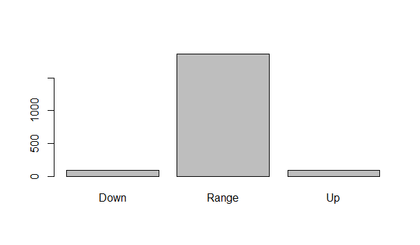
You can see most of the time the market is ranging. So just by predicting that the market is ranging, our model can make a correct prediction. But we will not be using this range prediction in our trading. We will be using the Up and down prediction in our trading. But as you can see in the above plot most of the time market in ranging and it moves up and down quite seldom. We need to be very accuracte about the Up and Down prediction. So we need to work more on the model. But I think we are working in the right direction and we can further improve our model using better deep learning models. Did you watch this documentary on UK Billionaire traders?